ENGINEERING ECONOMICS: A COMPREHENSIVE GUIDE

ENGINEERING ECONOMICS: A COMPREHENSIVE GUIDE

I. Basic Concepts and Definition of Terms: Engineering Economy and Accounting

Engineering Economy

• Focuses on evaluating the economic aspects of engineering and business projects.
• Involves assessing costs and benefits systematically.

Accounting

• Purpose: To record and summarize all financial transactions of a business.
• Goal: Provide accurate financial information to management for efficient operation.

Cost or Management Accounting

• Used for decision-making and control.
• Provides cost data crucial for engineering economy studies.

Types of Assets

• Fixed Assets: Long-term resources like buildings, machinery, and furniture.
• Current Assets: Short-term resources such as cash, accounts receivable, and inventory.
• Prepaid Expenses: Payments for services or materials not yet received.
• Intangible Assets: Non-physical assets like patents, copyrights, and trademarks.

Liabilities

• Fixed Liabilities: Long-term debts due after one year.
• Current Liabilities: Short-term obligations due within a year.

Ownership Types

• Sole Proprietorship: Single owner who may also manage the business.
• Partnership: Two or more individuals sharing ownership and management.
• Corporation: Ownership is divided into shares of stock; a separate legal entity.

Equities

• Claims against the assets of the enterprise, including liabilities and owner’s claims.

Financial Statements

• Balance Sheet: Shows assets, liabilities, and ownership equity at a specific date.
• Profit and Loss Statement: Summarizes income and expenses over a period to determine profit or loss.

Income Types

• Operating Income: Earnings from the core business activities.
• Non-Operating Income: Earnings from secondary activities like asset sales.

Expense Types

• Operating Expenses: Costs directly related to primary business operations.
• Non-Operating Expenses: Costs related to secondary activities not central to the business’s main operations.

Summary of financial ratios and their interpretation:

Ratio	Calculation	Meaning
Liquidity ratios
Current ratio	Current assets Current liabilities	The extent to which a firm can meet its short-term obligations.
Acid test or Quick      Ratio	Current assets-inventory Current liabilities	The extent to which a firm can meet its short-term obligations without relying upon the sale of its inventories.
Leverage ratios
Debt-to-total assets    Ratio	Total debt Total seets	The percentage of total finds that are provided by creditors.
Debt-to-equity ratio	Total debt Total stockholders’ equity	The percentage of total funds provided by creditors versus by owners.
Activity ratios
Inventory turnover	Sales Inventory of finished goods	Whether a firm holds excessive stocks of inventories and whether a firm is selling its inventories slowly compared to the industry average.
Fixed assets    turnover	Sales Fixed assets	Sales productivity and plant and equipment utilization.
Average collection    period	Accounts receivable Total sales/365 days	The average length of time, in days, it takes a firm to collect on credit sales
Profitability ratios
Gross profit margin	Sales-cost of goods sold Sales	The total margin available to cover operating expenses and yield a profit
Net profit margin	Net income Sales	After-tax profits per peso for sales.
Return on total assets (ROA)	Net income Total assets	After-tax profits per peso of assets, the ratio is also called return on investment (ROI).
Return on stockholders’  equity (ROE)	Net income Average stockholder’s equity	Afer-tax profits per peso of stockholders’ investment in the firm.
Earnings per share    (EPS)	Net income Number of shares of common stock outstanding	Earnings available to the owners of common stock.
Growth ratios
Sales	Annual percentage growth in sales.	Firm’s growth rate in sales.
Income	Annual percentage growth in profits	Firm’s growth rate in profits.
Dividends per share	Annual percentage growth in dividends per share	Firm’s growth rate in dividends per share.

II. Economic and Cost Concepts

Economics

• Definition: Study of production, distribution, and consumption of goods and services, and the interaction between people and wealth.

Market Structures

• Perfect Competition: Many sellers; no barriers to entry.
• Perfect Monopoly: Single seller; barriers prevent other sellers.
• Oligopoly: Few sellers; actions of one affect others.

Utility and Value

• Utility: Satisfaction a good or service provides.
• Value: Worth assigned to an item; often reflected in its price.

Types of Goods

• Consumer Goods: Directly satisfy wants (e.g., hamburger, haircut).
• Producer (Capital) Goods: Used in production (e.g., lathes, bulldozers).

Costs

• First Cost (Initial Cost): One-time cost to start an activity (e.g., purchase price, installation).
• Operation and Maintenance Costs: Ongoing costs during an investment’s life (e.g., labor, materials).
• Fixed Costs: Unchanged by activity level (e.g., taxes, salaries).
• Variable Costs: Change with activity level (e.g., materials, labor).
• Incremental Cost: Additional cost for increasing output (e.g., educating an extra student).
• Recurring Costs: Regularly repeated costs (e.g., office rental).
• Non-Recurring Costs: One-time expenditures (e.g., real estate, plant construction).
• Direct Costs: Attributed to a specific output (e.g., materials for a chair).
• Indirect Costs: Not easily attributed to a specific output (e.g., maintenance).
• Overhead Costs: General operating costs not related to direct labor/material (e.g., utilities).
• Prime Cost: Sum of direct labor and direct materials costs in manufacturing.

Relationship between cost and production

The relationship between cost and production involves how costs change with varying levels of production output. Here are the key concepts:

1. Cost Components

Fixed Costs: Costs that do not change with the level of production (e.g., rent, salaries). They are spread over more units as production increases, reducing the fixed cost per unit.

Variable Costs: Costs that vary directly with the level of production (e.g., raw materials, direct labor). They increase as production increases and decrease when production decreases.

Total Cost: The sum of fixed and variable costs. It increases with higher production but at different rates depending on the fixed and variable components.

2. Cost Behavior

Economies of Scale: As production increases, the average cost per unit often decreases due to spreading fixed costs over more units and achieving operational efficiencies.

Diseconomies of Scale: At very high production levels, inefficiencies and increased management costs can cause the average cost per unit to rise.

Marginal Cost: The additional cost incurred by producing one more unit. It is important for decision-making and pricing strategies.

Average Cost: Total cost divided by the number of units produced. It includes both fixed and variable costs and can decrease with increased production due to economies of scale.

3. Production Efficiency

Production Function: Shows the relationship between input levels (e.g., labor, materials) and output. Helps in understanding how changes in inputs affect total and average costs.

Cost-Volume-Profit (CVP) Analysis: Analyzes how changes in cost and production volume impact profitability. Helps in determining pricing, production levels, and cost management strategies.

4. Cost Management

Break-Even Point: The production level at which total revenues equal total costs. It helps in understanding the minimum production required to avoid losses.

Fixed and Variable Cost Allocation: Understanding how fixed and variable costs contribute to total cost helps in budgeting, pricing decisions, and financial planning.

By understanding these relationships, businesses can better manage production costs, optimize operations, and improve profitability.

Cost Types

Standard Costs: Predetermined costs per unit of output, established before actual production or service delivery.

Cash Cost: Involves actual cash payment and affects cash flow.

Book (Non-Cash) Cost: No cash transaction; reflected in accounting records (e.g., depreciation).

Sunk Cost: Past cost with no relevance to future decisions (e.g., non-refundable deposit).

Opportunity Cost: Cost of the best alternative foregone (e.g., income lost by attending school).

Life-Cycle Cost: Total costs associated with a product or service over its entire lifespan.

Working Capital: Funds required for current assets needed to support operational activities.

Disposal Cost: Non-recurring costs associated with shutting down operations and disposing of assets (e.g., site cleanup).

Relationship between total revenue and total cost

1. Definitions

Total Revenue (TR): The total income generated from selling goods or services. It is calculated as:

Total Revenue =Price per Unit × Quantity Sold

Total Cost (TC): The overall cost incurred to produce and sell goods or services. It includes both fixed costs (FC) and variable costs (VC). It is calculated as:

Total Cost = Fixed Costs + Variable Costs

where:

Variable Costs = Variable Cost per Unit × Quantity Produced

2. Profit and Loss

Profit (π): The financial gain or loss resulting from business operations, calculated as:

Profit=Total Revenue − Total Cost

Positive Profit: When Total Revenue exceeds Total Cost, indicating a gain.

Loss: When Total Revenue is less than Total Cost, indicating a loss.

3. Break-Even Analysis

Break-Even Point: The production level at which Total Revenue equals Total Cost. At this point, the business neither makes a profit nor incurs a loss. It can be calculated as:

• $$\text{Break-Even Point (in units)} = \frac{\text{Fixed Costs}}{\text{Price per Unit} - \text{Variable Cost per Unit}}$$

4. Cost-Volume-Profit (CVP) Analysis

Contribution Margin: The difference between the Price per Unit and Variable Cost per Unit. It is used to analyze how changes in production volume affect profitability:

Contribution Margin =  Price per Unit − Variable Cost per Unit

Contribution Margin Ratio: The proportion of each sales dollar that contributes to covering Fixed Costs and generating Profit:

• $$\text{Contribution Margin Ratio} = \frac{\text{Contribution Margin}}{\text{Price per Unit}}$$

5. Graphical Representation

Total Revenue Curve: Typically, this is a straight line starting from the origin with a slope equal to the Price per Unit.

Total Cost Curve: Starts from the Fixed Costs (vertical intercept) and increases linearly with the slope equal to the Variable Cost per Unit.

Intersection Point: The point where the Total Revenue curve intersects the Total Cost curve is the Break-Even Point.

6. Margin of Safety

Margin of Safety: The difference between actual or projected sales and the Break-Even Sales. It indicates the risk level of incurring a loss:

• $$\text{Margin of Safety} = \text{Actual Sales} - \text{Break-Even Sales}$$
  

7. Profitability Analysis

• Profitability: A business’s ability to generate profit is assessed by how Total Revenue exceeds Total Cost over different production levels. Analyzing changes in Total Revenue and Total Cost helps in making pricing, production, and strategic decisions to enhance profitability.

Understanding the interplay between Total Revenue and Total Cost helps businesses manage their finances effectively, make informed decisions, and strategize for growth and sustainability.

Common Methods of Allocating Factory Indirect Charges to the Product Being Produced:

    a. Direct-labor-cost method

    b. Direct-labor-hour method

    c. Direct-material-cost method

Cost driven design optimization is a procedure for determining optimal design using cost concepts.

Present economy studies are cost analyses undertaken when the influence of time on money is not a significant consideration.

III. Interest Factor Formulas and Equivalence Calculations

    • Capital is wealth in the form of money or property that is capable of being used to produce more wealth.

    • Equity capital is that owned by individuals who have invested their money or property in a business project in the hope of receiving a profit.

    • Debt or borrowed capital is obtained from lenders who receive interest in return from the borrowers.

    • Interest is a fee that is charged for the use of someone else’s money.  The percentage of money charged as interest is called interest rule.

    • Simple interest  is defined as a fixed percentage of the principal (initial amount of loan or money borrowed) multiplied by the life of the loan (or the number of interest periods for which the principal is committed).

    • Compound interest is charged whenever the interest for any interest period is calculated based on the remaining principal amount plus any accumulates interest charges up to the beginning of that period.

    • Principal or present sum of money is the equivalent worth of one or more cash flows at a reference point in time called the present.

    • Compound amount or future sum of money is the equivalent worth of one or more cash flows at a reference point in time called the future.

    • A cash flow is the difference between total cash receipts (inflows) and total cash disbursements (outflows) expenditures for a given period of time.

    • A cash flow diagram is used to visualize a cash flow individual cash flows are presented as vertical arrows along a horizontal time scale.

Example of a cash flow diagram

End-of-period	Event or transaction
0 (now)	Outlay of P100,000
1	Additional expenditure of P25,000
2	Receipt of P60,000
3 to 6	Uniform Receipts of P80,000
7	Receipt of P100,000

     

Cash flow diagram (CFD):

    • Discrete compounding means that the interest is compounded at the end of each finite length period, such as a month or a year.

    • Single payment, compound amount factor is used to float F when given P. – It is given by

                 F = P(1 + i)ⁿ = P x (F/P, i, n)

    • Single payment, present worth factor is used to find P when given F – It is the reciprocal of the compound amount factor and is given by

                    P = F(1 + i)ⁿ = F x (P/F, i, n)

• Uniform series  means uniform amount of money, A, occurring at the end of each period of a periods with interest at 1% per period.  A uniform series is often called annuity.

Other assumptions:

a. P (present worth) occurs at 1 interest period before the first A.

b. F (future worth) occurs at the same time as the last and n interest periods after P.

c. A (annual worth) occurs at the end of periods 1 through n, inclusive.

    • Uniform series, compound amount is used to find F when given A – It is given by

    • Uniform series, present worth factor is used to find P when given A – It is given by

    • Uniform series, sinking fund factor is used to find A when given F. – It is the reciprocal of the uniform series compound amount factor and is given by

    • Uniform series, capital recovery factor is used to find A when given P.  – It is the reciprocal of the uniform series present worth factor and is given by

    • A uniform gradients series is a series of annual payments in which each payment is greater than the previous one by a constant amount, G.

    • Uniform gradient series factor is used to find A when G is given. – It is expressed as

    • A geometric gradient  is one where annual cash flows increase or decrease over time by a constant percentage g. If F1 is the payment at the end of year 1, the magnitude of payment during the nth year is given by

F_n = F₁(1 + g)^n-1

    Note:  When g is positive, the series will increase.  When g is negative, the series will decrease.

    • Geometric gradient series factor is used to find P when a geometric gradient series is given.  It can be expressed as

    • Ordinary annuities are uniform amounts in which the first cash flow is made at the end of the first period.

    • Economic equivalence means that different sums of money at different times can be equal in economic value.  Economic equivalence is established, in general, when we are indifferent between a future payment, or series of future payments, and a present sum of money.

    • The nominal interest rate (r per year) or the basic annual interest rate is a customary way of stating interest rate, as in 12% compounded semiannually, where 12% is the nomimal rate per year.

    • Effective annual rate, i_a, is the actual or exact rate of interest earned on the principal during one year.  Note that it is always expressed on an annual basis.

The relationship between effective annual interest, i_a, and nominal interest r, is

 i_a = (1 + r/M)^M – 1

           where:  M is the number of compounding periods per year and r is expressed in decimal

Table 2.  Various interest statements and their interpretation.

Interest rate statement	Interpretation	Comment
i = 12% per year i = 1% per month i = 3 ½% per quarter	i = effective 12% per year compounded yearly i = effective 1% per month compounded monthly i = effective 3 ½% per quarter compounded quarterly	When no compounding period is given, interest rate is an effective rate, with compounding period assumed to be equal to stated time period.
i = 8% per year, compounded monthly   i = 4% per quarter compounded monthly   i = 14% per year compounded semiannually	i = nominal 8% per year compounded monthly   i = nominal 4% per quarter compounded monthly   i = nominal 14% per year  compounded semiannually	When no compounding period is given without stating whether the interest rate is nominal or effective, it is assumed to be nominal.  Compounding period is as stated.
i = effective 10% per year compounded monthly   i = effective 6% per            quarter   i = effective 1% per month compounded daily	i = effective 10% per year compounded yearly   i = effective 6% per quarter compounded quarterly   i = effective 1% per month  compounded daily	If interest rate is stated as an effective rate, then it is an effective rate.  If compounding period is not given, compounding period is assumed to coincide with stated time period.

Table 3.  Specific examples of interest statements and interpretations

Interest statement	Type of Interest	Compounding period
15% per year compounded monthly 15% per year Effective 15% per year compounded monthly 20% per year compounded quarterly Nominal 2% per month compounded weekly 2% per month 2% per month compounded monthly Effective 6% per quarter Effective 2% per month compounded daily 1% per week compounded continuously 0.1% per day compounded continuously	Nominal Effective Effective Nominal Nominal Effective Effective Effective Effective Nominal Nominal	Monthly Yearly Monthly Quarterly Weekly Monthly Monthly Quarterly Daily Continuously Continuously

Source; Blank and Tarquin.  1989.  Engineering Economy (3rd ed. ) McGraw-Hill International.

    • A bond is a financial instrument setting forth the conditions under which money is borrowed.

    • Par value or face value is the value stated on the bond (as in a check, note, bill or other paper security), usually in multiplies of P1,000,

    • A bond’s yield to maturity is the effective annual interest rate earned by a bond, taking into consideration periodic interest payments and disposal or redemption price of the bond at maturity.

    • Maturity refer to the time that a bond or note is payable.

    • A bond’s current yield also known as coupon rate, is the interest earned each year as a percentage of the bond’s purchase price.

    • A bond also earns a bond rate representing interest per interest period, generally stated as a nominal rate per interest period, and is calculated based on the par or face value.

    • Stock represents a share of ownership in a company.

    • Working capital refers to additional funds to finance any cash needs, accounts receivables, or inventories that arise from investment make into a new project.  It is comprised o short-term or current assets that include cash, customer’s unpaid bills, inventories of raw materials, work-in process, and finished goods.

    • Continuous compounding assumes that cash flows occur at discrete intervals but that compounding is continuous throughout the interval.

IV. Methods of Evaluating Alternatives

    • Minimum attractive rate of return (MARR) is the rate of return chosen by top management of an organization to maximize its economic well-being.  It is also known by many other names such as hurdle rate, target rate, cut-off rate, discount rate or valuation rate.

    • Present Worth (or Net Present Value, NPV) expresses the equivalent worth of all cash flows relative to some base or beginning point in time called the present.  It can be found using the following relationship.

PW (i%) = F_o(1 + i)^o + F₁(1 + i)^-1 + F₂(1 + i)² + …+ F_k(1 + i)^k + … + F_n(1 + i)^-n

            or

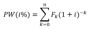
            where:

                         i = effective interest rate, or MARR, per compounding period

              k = index for each compounding period (0 £ k £ n)

            F_k = future cash flow at the end of period k

              n = number of compounding periods in the planning horizon

Criterion: A project is acceptable if PW ³ 0.

    • Future Worth expresses cash inflows and outflows are compounded forward to a reference point in time called the future.  To determine the future worth of a project, the following relationship is used:

FW (i%) = F_o(1 + i)ⁿ + F₁(1 + i)^n-1 + … + F_n(1 + i)⁰

or

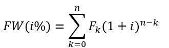
 Criterion:  A project is acceptable if FW ³  0.

    • The annual worth is the annual equivalent revenues (or savings).  R, minus annual equivalent expenses, E, less its annual equivalent capital recovery cost, CR.

    -AW is calculated as follows:

                                            AW(i%) = R – E – CR (i%)

    • Capital Recovery (CR) cost is computed with i = MARR using the following equation:

                                         CR (i%) = I x (A/P.1% n) – S x (A/F, i%, n)

                 where  I = initial investment for the project

                            S = salvage (residual) value at the end of the study period

                            n = project study period.

          Criterion: A project is acceptable if AW ³ 0.

    • Internal Rate of Return is the most widely used method, and is also known as investor’s method, discounted cash flow method, and profitability index.  This involves solving for the interest rate, termed internal rate of return (IRR), that equates the equivalent worth of cash inflows (receipts or savings) to the equivalent worth of cash outflows (expenditures, including investments).

    By using a PW formulation, IRR is the i% at which

             

        where:  R = net revenues or savings for the kth year

                     E = net expenditures including investments for the kth year

                     n = project life (or study period)

                  Criterion:  A project is acceptable if i% > MARR.

    • Benefit/Cost Ratio is also known as savings-investment ratio (SIR) Two commonly used formulations of the B/C ratio (expressed in terms of AW) are:

1. Conventional B/C ratio

                   

                   where AW = annual worth

                              B  = annual equivalent worth of benefits of the proposed project

                             CR = capital recovery cost

                       O & M = equivalent annual operating and maintenance expenses of the proposed project

2. Modified B/C ratio:

 The numerator expresses the equivalent worth of the benefits minus the equivalent annual operating and maintenance costs.  The denominator includes only the annual equivalent investment costs.

 Criterion:  A project is acceptable when either the conventional or modified B/C ratio is greater than or equal to 1.0.

• Payback Period, also called the simple payout period, mainly indicates a project’s liquidity rather than its profitability.  It has been used as a measure of a project’s risk, since liquidity deals with how fast an investment can be recovered.  The payback method calculates the number of years required for positive cash flows to just equal the total investment, P.  The simple payback period is the smallest value of a for which the relationship below is satisfied under end-of-year cash flow convention.

The simple payback period n ignores the time value of money and all cash flows that occur after n.  The discounted payback period, n’, is calculated to take into consideration the time value of money as follows:

• The capitalized equivalent amount (capitalized worth) of a project is the present worth or value of a project that is assumed to last forever. If only expenses are considered, results obtained are appropriately expressed as capitalized cost.  The capitalized worth method is a convenient basis for comparing mutually exclusive alternatives when the period of needed service is indefinitely long.

Given a perpetual annual uniform payment, A, with interest at 1% per period, the capitalized equivalent amount (CEA) or capitalized worth (CW) is:

                  CEA = P = A(^{P/A, i%, µ}).

                   As n becomes very large. (^{P/A, i%, n}) è l/i

                   Thus CEA = P = A(l/i)

• Rate of return (ROR) on capital invested is given by the formula:

ROR is used as a measure of the effectiveness of an investment of capital.  It is an indicator of financial efficiency.  When this method is used, it is necessary to decide whether the computed rate of return is sufficient to justify the investment.

V. Decision-Making Among Investment Alternatives

    • An investment alternative is a decision option.  It can consist of a group or a set of proposals.

    • An engineering proposal is a single undertaking or project being considered as an investment possibility.

    • A proposal is said to be independent when the acceptance of the proposal from a set has no effect on the acceptance of any of the other proposals in the set.

    • Proposals are said to be mutually exclusive if the acceptance of one proposal from the set precludes the acceptance of any of the others.

    • Auxiliary proposals are called contingent proposals because their acceptance is conditional on the acceptance of another proposal, also called the prerequisite proposal.

As a policy.  “The alternative that requires the minimum investment of capital and produces satisfactory functional results will be chosen among mutually exclusive alternatives unless the incremental capital associated with an alternative having a larger investment can be justified with respect to its incremental savings (or benefits)”.

• The base alternative is the alternative that requires the least investment of capital and that has a return equal to or greater than the MARR.  The investment of additional capital over the base alternative should be made if the extra benefits, for example, increased capacity, increased quality, increased revenues, decreased operating expenses, or increased life are better than those that could be obtained from investment of the some capital elsewhere.

• Investment alternatives are those with initial or (front-end) capital investment(s) that produce cash flows from increased revenue, savings through reduced costs, or both.

• Cost alternatives are those with all negative cash flow elements except for a possible positive cash flow element from disposal of assets at the end of the project’s life.

Procedure for Comparing Two Alternatives

 Choosing between two alternatives can be performed by incremental investment analyses as follows:

1.     With the lower initial cost alternative as base alternative, i.e., as alternative (A) tabulate cash flow for both alternative in the order of increasing initial investment.

2.    Calculate the difference, D(B-A) (or incremental net cash flow A ® B, where the arrow means file increment between Alternative A and B).

3.    Draw an incremental net cash flow diagram.

4.    Determine the present worth (PW_A®B), the internal rate of return (IRR_A®B), or any appropriate measure of merit, of the incremental cash flow.

5.    If PW_A®B is greater than O, or if IRR_A®B is greater than the MARR, then the incremental investment is justified and select B, otherwise, select A.

When alternatives have unequal lives, a procedure that v   put the alternatives on a comparable basis must be adopted before making an engineering economy study.  The do this, two assumptions regarding the study period can be employed.

a. Repeatability assumption.  This involves 2 conditions:

    i. Study period over which the alternatives are compared is either indefinitely long or equal to a common multiple of the lives of the alternatives (Use least common multiple to present worth comparisons).

    ii. Economic consequences that are estimated to happen in alternative’s life span will also happen in all succeeding life spans, if any.

b. Coterminal assumption.   It uses a selected study period for all alternatives, with appropriate assumptions and adjustments to put alternatives on a common and comparable basis.

Steps in the incremental investment analysis procedure for comparing more than two mutually exclusive alternatives:

1. Arrange (order) the alternatives based on increasing initial investment cost.

2. Establish a base alternative.

Among cost alternatives, the first alternative with the least initial investment cost is the base.  For investment alternatives, if the selection criterion value for first alternative is acceptable, select it as the base; otherwise, select the next alternative in the arranged order.  Continue until an acceptable criterion value is obtained.

3. Use iteration to evaluate differences between alternatives until no more alternatives exist.

    3.1 If the criterion value for the incremental cash flow between the next alternative and the current best alternative is favorable; choose the next alternative as the current best alternative.  Otherwise, retain the last alternative with an acceptable criterion value as the current best alternative.

    3.2 Repeat and select as the preferred alternative the last one for which the incremental cash flow criterion value was acceptable.